Aperture Efficiency

The ``aperture efficiency'' of an antenna was earlier defined (Sec 19.3) to be the ratio of the effective radiating (or collecting) area of an antenna to the physical area of the antenna. The aperture efficiency of a feed-and-reflector combination can be decomposed into five separate components: (i) the illumination efficiency or ``taper efficiency'', ${{\eta}_t}$, (ii) the spillover efficiency, ${{\eta}_S}$, (iii) the phase efficiency, ${{\eta}_p}$, (iv) the crosspolar efficiency, ${{\eta}_x}$ and (v) the surface error efficiency ${{\eta}_r}$.

$${{\eta}_a} = {{\eta}_t}\:{{\eta}_S}\:{{\eta}_p}\:{{\eta}_x}\:{{\eta}_r}.$$ (19.4.10)

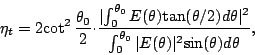
The illumination efficiency (see also Chapter 3, where it was called simply ``aperture efficiency'') is a measure of the nonuniformity of the field across the aperture caused by the tapered radiation pattern (refer Figure 19.2). Essentially because the illumination is less towards the edges, the effective area being used is less than the geometric area of the reflector. It is given by

$${{\eta}_t} = \frac{\vert\int_{0}^{R} g(r) dr\vert^2}{\int_{0}^{R} \vert g(r)\vert^2 dr}, \\$$ (19.4.11)

where $g(r)$ is the aperture field. Note that this has a maximum value of 1 when the aperture illumination is uniform, i.e. $g(r)=1$. The illumination efficiency can also be written in terms of the electric field pattern of the feed $E(\theta)$, viz.

$${{\eta}_t} = 2{\cot^2{\frac{{\theta}_0}{2}}}{\cdot}{\frac{\... ..._0}{\vert E({\theta})\vert^2{\sin({\theta})}d{\theta}}}}, \\$$ (19.4.12)

where ${{\theta}_0}$ is angle subtended by the edge of the reflector at the focus (Figure 19.1).

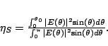
When a feed illuminates the reflector, only a proportion of the power from the feed will intercept the reflector, the remainder being the spillover power. This loss of power is quantified by the spillover efficiency, i.e.

$${{\eta}_S} = {\frac{\int_{0}^{{\theta}_0}{\vert E({\theta... ...pi}{\vert E({\theta})\vert^2{\sin({\theta})}d{\theta}}}}. \\$$ (19.4.13)

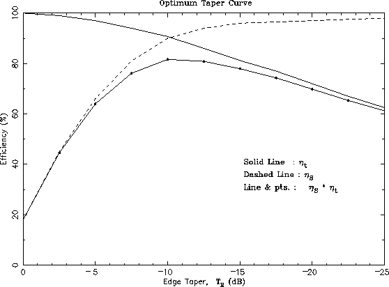
Note that the illumination efficiency and the spillover efficiency are complementary; as the edge taper increases, the spillover will decrease (and thus ${{\eta}_S}$ increases), while the illumination or taper efficiency ${{\eta}_t}$ decreases^19.1 The tradeoff between ${{\eta}_S}$ and ${{\eta}_t}$ has an optimum solution, as indicated by the product ${{\eta}_S}$ * ${{\eta}_t}$ in Figure 19.3. The maximum of ${{\eta}_S}{{\eta}_t}$ occurs for an edge taper of about -11 dB and has a value of about 80 %. In practice, a value of -10 dB edge taper is frequently quoted as being optimum.

Figure 19.3: Illumination efficiency and spillover efficiency as a function of edge taper. The optimum taper is at $\sim -11$ dB.

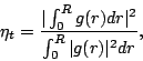
The surface-error efficiency is independent of the feed's illumination. It is associated with far-field cancellations arising from phase errors in the aperture field caused by errors in the reflector's surface. If ${\delta}$ is the rms error in the surface of the reflector, the surface-error efficiency is given by

$${ {\eta}_r} = {\exp{-(4{\pi}{\delta_p}/{\lambda})^2}}$$ (19.4.14)

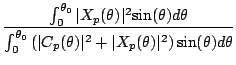
The remaining two efficiencies, the phase efficiency and the cross polarization efficiency, are very close to unity; the former measures the uniformity of the phase across the aperture and the latter measures the amount of power lost in the cross-polar radiation pattern. For symmetric feed patterns[6], ${{\eta}_x}$ is defined thorough the copolar, ${C_p}({\theta})$ and cross-polar patterns, ${X_p}({\theta})$:

$${{\eta}_x} = {\frac{\int_{0}^{{\theta}_0}{\vert{X_p}({\theta})\vert^2{\sin( {\... ...theta})\vert^2+ \vert{X_p}({\theta})\vert^2 \right){\sin({\theta})}d{\theta}}}}$$ (19.4.15)

where,

$${C_p}({\theta}) = 1/2[E({\theta}) + H({\theta})]$$ (19.4.16)

$${X_p}({\theta}) = 1/2[E({\theta}) - H({\theta})]$$

It can be seen that if one can design an antenna,having identical $E({\theta}),H({\theta})$ patterns the cross-polar pattern will vanish. Taking the cue from this, the feed for antenna could also designed with a goal to match E and H patterns at least up to the subtended angle of the dish edge, $\:{{\theta}_0}$.

With this background we now proceed to take a detailed look at the GMRT antennas.

Footnotes

... decreases^19.1

Recall also from Chapter 3 that as the illumination is made more and more uniform the sidelobe level increases.